A Story of the Determinant of Operator-Valued Semicircular Elements

Operator-valued semicircular elements are the powerhouse of free probability and random matrix theory. In particular, the intrinsic freeness principle typically replaces random matrices by operator-valued semicircular elements and shows that, in many respects, the former are close to the latter. Thus it is important to understand as much as possible about operator-valued semicirculars.

An operator-valued semicircular element – say over $B=M_m(\mathbb C)$ – is of the form

S=a\otimes 1+\sum_{i=1}^n a_i\otimes s_i\qquad\text{with} \qquad a,a_1,\dots,a_n\in M_m^{sa}(\mathbf C),

where $s_1,\dots,s_n$ are free semicirculars. We denote by ${\rm tr}_m$ the normalized matrix trace on B, and by $\tau$ the trace on the algebra, where the $s_i$ live. All information about such an element S is contained in its

\text{mean} \quad ({\rm id} \otimes \tau)[S]=a \qquad \text{and its covariance}\quad \eta(b)=:({\rm id}\otimes \tau)[(S-a)b(S-a)]=\sum_{i=1}^n a_i b a_i.

The covariance is a completely positive map from B to B.

We also know how, in principle, to calculate the distribution $\mu_S$ of S. Its scalar-valued Cauchy transform is

g_S(z)=(\tr_m\otimes \tau)[(z1-S)^{-1}].

This can be extracted from the operator-valued Cauchy transform

G_S(b)=({\rm id}\otimes\tau)[(b-S)^{-1}]

simply by

g_S(z)=\tr_m[G_S(z1)].

And $G_S$ is determined by the nice quadratic matrix-valued equation, usually called the Dyson equation,

(b-a)\cdot G_S(b)=1+\eta(G_S(b))\cdot G_S(b).

So everything is determined by mean and covariance. Of course, some quantities are easier, others harder to extract in a meaningful way. For moments of S, for example, one has the operator-valued free version of the Wick/Isserlis formula. The operator norm of S, on the other hand, is not so easily accessible. In principle, this is given by the asymptotics of high moments, but that is not very concrete. So the following celebrated formula of Franz Lehner

\lambda_{\max} \left(a\otimes 1+\sum_{i=1}^n a_i\otimes s_i\right) = \inf_{b\in B, b \gt 0}\lambda_{\max} \left(b+a+\eta(b^{-1})\right)

comes as a nice surprise, as it reduces the upper spectral edge of the infinite-dimensional S to a variational problem for the same quantity on the finite-dimensional B. Here $\lambda_{\max}$ denotes the upper edge of the spectrum; for positive $a$ , Lehner’s original formulation gives the corresponding operator norm.

A few years ago together with Tobias Mai I was trying to understand the determinant (more precisely, the Fuglede–Kadison determinant) of an operator-valued semicircular element, in order to get some info about the accumulation of mass of the distribution of such a semicircular element close to zero. And we succeeded in finding a nice formula in terms of the covariance; more precisely the determinant was essentially given by the capacity of the covariance map. Capacity here is the quantity introduced by Gurvits in connection with operator scaling; it should not be confused with the various notions of channel capacity in quantum information. Unwinding this notion of capacity one can write our result concretely as

\Delta(\sum_{i=1}^n a_i\otimes s_i) = e^{-1/2}\cdot \inf_{b\in B, b>0} \Delta\left(b\cdot \eta(b^{-1})\right)^{1/2}.

$\Delta$ is here the Fuglede–Kadison determinant, which reduces in the finite-dimensional situation to

\Delta(b)=\det (\vert b\vert)^{1/m}\qquad\text{for}\qquad b\in M_m(\mathbb C).

As you see, our result is only for mean a=0. But in this case it has a striking similarity with Lehner’s formula:

\| \sum_{i=1}^n a_i\otimes s_i\| = \inf_{b\in B, b>0} \left\|b+\eta(b^{-1})\right\|,

And of course it raises the question: Can we extend our formula also to the case of general mean. We thought a little bit about this way back then, but did not see how to do this.

Now, in the times of AI hype, it is tempting to come back to this question and ask ChatGPT what it has to say on this. And actually, it has something to say. It proposes the following generalization

\Delta\left(a\otimes 1+\sum_{i=1}^n a_i\otimes s_i\right) = e^{-1/2} \inf_{b \gt 0,\ \mathcal C_b-\eta\succeq 0} \Delta(b)\, \exp\left\{ \frac12 \left\langle a, (\mathcal C_b+\eta)^{-1}(a) \right\rangle_2 \right\},

where

\mathcal C_b(x)=bxb,\qquad\text{and}\qquad\langle x,y\rangle_2 = \operatorname{tr}_m(x^*y)\qquad \text{for} \qquad x,y\in M_m(\mathbb C)

is the Hilbert-Schmidt inner product.

The condition $\mathcal C_b-\eta\succeq 0$ means positivity as an operator on the Hilbert–Schmidt space $M_m(\mathbb C)$ , i.e.

\left\langle x,\mathcal C_b(x)\right\rangle_2 \geq \left\langle x,\eta(x)\right\rangle_2,\qquad\text{or equivalently}\qquad \operatorname{tr}_m(x^*bxb) \geq \operatorname{tr}_m\left(x^*\eta(x)\right), \qquad\text{for all }x\in M_m(\mathbb C).

ChatGPT also produces what it claims is a proof of all this — note that even the reduction of this to my formula with Tobias in the case of a=0 is non-trivial — and makes some remarks on the relevance for the Brown measure of an operator-valued circular element. Recall that the Brown measure of an operator $T$ is encoded by the logarithmic potential

z\mapsto \log \Delta (T-z1).

So understanding determinants of shifted operators is exactly what one needs here.

All this looks somehow reasonable, but not very enlightening; and even if I had a Lean certificate for all this (which I don’t), I would still not be too satisfied.

So let’s talk about all this and hope that, together, we can get a better understanding of what is really going on.

Doing Mathematics with AI — but How?

Leave a reply

AI is revolutionizing mathematics, and it will not go away. So somehow we have to arrange ourselves with it and find our way of doing mathematics under these changed conditions.

I am of course also fascinated by asking AI (ChatGPT in my case) to solve all my problems. And sometimes there are indeed answers which seem to be okay and which promise some real progress. But those answers are usually complicated and quite technical, and I don’t really feel like becoming a little helper and argument checker for AI.

I agree with many voices saying that asking the meaningful questions, and understanding and presenting the answers, will remain some of the main tasks for us. But this should happen in a way that we still feel good about going along with it. For me this means that I would like to take from AI mainly some ideas, but then think myself about whether they could be true, what they actually mean, how one could prove them, and what is the best way to present them and convince others.

Of course, like everybody else, I don’t have a final answer to how this should work in practice, or whether this is a route which will help mathematics to survive in anything resembling its present form.

Anyhow, I suppose we just have to try different routes. Here is one experiment I would like to make.

At the moment I am thinking about determinants of operator-valued semicircular elements. Together with Tobias Mai, we derived a few years ago a formula for the determinant of such an element S in terms of its covariance map. This was, however, for the case of vanishing mean of S, and I wondered whether there could be a nice and useful extension to the case of general mean.

Okay, so I asked ChatGPT. And it did what two years ago would have seemed totally out of range, but has now become almost ordinary: it gave me an answer, proved it, and also made some comments on possible implications for questions about the Brown measure of operator-valued circular elements.

It even wrote a manuscript about all this.

I could now just put my name on it, say that the ideas were developed in conversations with AI, and declare that I take full responsibility for the results. But this does not feel right to me. And, more importantly, it does not feel very satisfying.

So here is what I would rather like to do.

I will give some background, explain what ChatGPT proposes as the answer, and then open the problem for public discussion: Is the statement correct? Is it perhaps obvious? How is it related to things that somebody already knows? What is the right proof? And what other interesting questions or conjectures might come out of it?

My dream would be that the answers — and also the questions — are actually self-thought, and not just copies of something another AI conversation produced. Of course everybody could now ask AI about the problem and perhaps produce a paper on it. But this should not be about publishing or priority. It should be about understanding.

Maybe one could think of it as telling a mathematical story together, in a somewhat grassroots way: somebody starts with a question, somebody else recognizes a connection, another person finds an argument, somebody points out that the whole thing is wrong, or suggests the right formulation, and gradually we understand what is really going on. Of course, we can use AI in the background for information, references, or inspiration. But AI should not tell the story.

I have no idea whether this will work.

But let us try.

In my next post I will give the concrete mathematical problem and the beginning of the story.

The intermediate quantum permutation group problem

2 Replies

Guest post by Amaury Freslon

At a recent conference celebrating Roland Speicher’s birthday, I gave a talk on a problem from the theory of compact quantum groups that has fascinated me for years and on which Roland and I have been working, albeit unsuccessfully. I wrote detailed notes introducing the problem, which are available here and Roland suggested I write a blog post to publicize them. So here I am !

Let’s begin by unpacking the terminology in the title. The quantum permutation group S_N⁺, introduced by Sh. Wang, is defined via a universal ∗-algebra 𝒪(S_N⁺), which is generated by entries of a matrix (p_ij). These entries are subject to relations that resemble those of classical permutation matrices, but with the key difference that they do not commute. More precisely, the defining properties are as follows:

Each generator is idempotent and self-adjoint;
They are pairwise orthogonal on rows and columns;
They add up to 1 on rows and columns.

In contrast, let 𝒪(S_N) be the algebra of all complex-valued function on the classical permutation group S_N. The connection between S_N⁺ and S_N is given by a canonical ∗-homomorphism π_ab: 𝒪(S_N⁺) → 𝒪(S_N), which is defined by making all generators commute. In that sense, S_N⁺ can be thought of as the free or quantum version of S_N. We can now state our main problem:

Does there exist a compact quantum group 𝔾 such that S_N<𝔾<S_N⁺? In other words, is there a Hopf ∗-algebra 𝒪(𝔾) through which the map π_ab factors?

In algebraic terms, the problem asks whether there exists a non-trivial Hopf ideal inside the commutator ideal of 𝒪(S_N⁺). However, understanding Hopf ideals in general is notoriously difficult, so we must look for alternative approaches. One promising direction involves exploiting the fact that the quantum permutation group is an easy quantum groups in the sense that all the relations in the algebra 𝒪(S_N⁺) are encoded by partitions of finite sets. While we will not delve into the details here (see the notes and references therein), we can sketch a potential strategy.

The relations in 𝒪(S_N⁺) are exactly those given by linear combinations of non-crossing partitions;
The relations in 𝒪(S_N) are exactly those given by linear combinations of arbitrary partitions;
The problem therefore boils down to this: if we are given a relation corresponding to a linear combination of arbitrary partitions, can we combine it with relations coming from non-crossing partitions to obtain all possible relations from partitions?

While this approach seems reasonable, it has not proven efficient thus far. The only known results on the problem, which rely on different techniques, are as follows:

For N<4, there is no intermediate quantum permutation group, because S_N=S_N⁺ in that case;
For N=4, there is again no intermediate quantum permutation group, as can be observed on the complete list of quantum subgroups of S₄⁺;
For N=5, the absence of intermediate quantum permutation group was obtained by T. Banica relying on deep results from the classification of subfactors.

The notes outline an alternative approach developed by Roland Speicher and myself which is inspired by noncommutative probability theory. More precisely, any quantum subgroup 𝔾 of S_N⁺ comes with a distinguished linear form, known as its Haar state. Pulling it back to 𝒪(S_N⁺), we obtain a map with lots of symmetry properties coming from the fact that 𝔾 is assumed to contain S_N. One might therefore try to prove that such a highly symmetric state must coincide with the Haar state of S_N⁺ or with that of S_N, thereby answering negatively the question.

To tackle this, we focus on the moments of the Haar state, that is, its values on elements of the form x = p_i1j1p_i2j2...p_ikjk. These moments satisfy algebraic relations that arise from the ones satisfied by the generators, along with the symmetries induced by S_N. Using these, we were able to show that the moments of order up to 5 of such a state must either match the corresponding moments of S_N⁺, or those of S_N. Although this is encouraging, our method breaks down at order 6, were we encounter complicated systems of quadratic equations. Nonetheless, there is a glimmer of hope because it may be possible to incorporate an additional ingredient: the fact that the Haar state sends elements of the form x^*x to positive real numbers.

I hope that this motivates the reader to take a closer look at these notes and perhaps try their luck at the problem.

Understanding Non-Linearity in Random Matrices

Leave a reply

Update: I will give an online talk on my work with Alex in Voiculescu’s Probabilistic Operator Algebra Seminar on Monday, Feb 3, at 9am Pacific time (which is 6pm German time). In order to get the online link for the talk you should write to jgarzav at caltech dot edu.

In the post “Structured random matrices and cyclic cumulants: A free probability approach” by Bernard and Hruza I mentioned the problem about the effect of non-linear functions on random matrices and showed some plots from my ongoing joint work with Alexander Wendel. Finally, a few days ago, we uploaded the preprint to the arXiv.

What is this about? Consider a random matrix ensemble X_N which has a limiting eigenvalue distribution for N going to infinity. In the machine learning context applying non-linear functions to the entries of such matrices plays a prominent role and the question arises: what is the asymptotic effect of this operation. There are a couple of results in this direction; see, in particular, the paper by Pennington and Worah and the one of Peche. However, it seems that they deal with quite special choices for X_N, like a product of two independent Wishart matrices. In those cases the asymptotic effect of applying the non-linearity is the same as taking a linear combination of the X_N with an independent Gaussian matrix. The coefficients in this linear combination depend only on a few quantities calculated from the non-linear function. Such statements are often known as Gaussian equivalence principle.

Our main contribution is that this kind of result is also true much more generally, namely for the class of rotationally invariant matrices. The rotational invariance is kind of the underlying reason for the specific form of the result. Roughly, the effect of the non-linearity is a small deformation of the rotational invariance, so that the resulting random matrix ensemble still exhibits the main features of rotational invariance. This provides precise enough information to control the limiting eigenvalue distribution.

We consider the real symmetric case, that is, symmetric orthogonally invariant random matrices. Similar results hold for selfadjoint unitarily invariant random matrices, or also for corresponding random matrices without selfadjointness conditions.

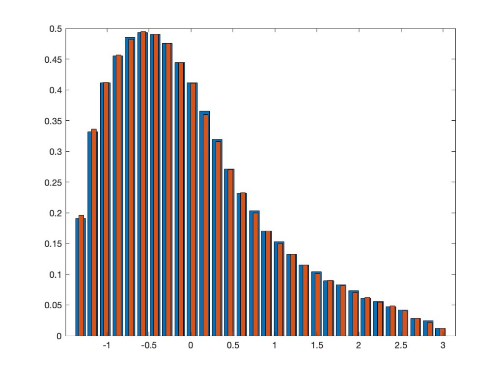
In addition to what I already showed in the above mentioned previous post, we extended the results now also to a multi-variate setting. This means we can also take, again entrywise, a non-linear function of several jointly orthogonally invariant random matrices. The asymptotic eigenvalue distribution after applying such a function is the same as for a linear combination of the involved random matrices and an additional independent GOE. As an example, take the two random matrices X_N=A_N²– B_N and Y_N=A_N⁴+C_NA_N+A_NC_N, where A_N, B_N, C_N are independent GOEs. Note that, by the appearance of A_N in both of them, they are not independent, but have a correlation. Nevertheless, they are jointly orthogonally invariant — that is, the joint distribution of all their entries does not change if we conjugate both of them by the same orthogonal matrix. We consider now the non-linear random matrix max(X_N,Y_N), where we take entrywise the maximum of the corresponding entries in X_N and Y_N. Our results say that asymptotically this should have the same eigenvalue distribution as the linear model aX_N+ bY_N + cZ_N, where Z_N is an additional GOE, which is independent from A_N, B_N, C_N, and where a, b, c are explicitly known numbers. The next plot superimposes the two eigenvalue distributions.

If you want to know more, in particular, why this is true and how the coefficients in the linear model are determined in terms of the non-linear function, see our preprint Entrywise application of non-linear functions on orthogonally invariant random matrices.

The noncommutative Edmonds’ problem revised: how to calculate the inner rank of matrices in noncommuting variables

Leave a reply

Update: The paper has now been published in Foundations of Computational Mathematics as an open access article. Here is a link.

My paper with Johannes and Tobias on the noncommutative Edmonds’ problem has got a total makeover; the new revised version appeared just on the arXiv. It relies now heavily on the recent results of Tobias and mine on the Fuglede-Kadison determinant of matrix-valued semicircular elements. But also, the organization of the paper is now much more reader-friendly – at least we hope so. Everything you need to know can be gotten from the first three sections; if you need proofs, read the rest.

Let me first recall the noncommutative Edmonds’ problem. Consider a matrix

$A=a_1\otimes x_1+\ldots+a_n\otimes x_n$ ,

where the $x_i$ are noncommuting variables and the $a_i$ are arbitrary matrices of the same size N; N is fixed, but arbitrary.

The noncommutative Edmonds’ problem asks whether A is invertible over the noncommutative rational functions in the $x_i$ ; this is equivalent (by deep results of Cohn) to asking whether A is full, i.e., its noncommutative rank is equal to N. The noncommutative rank is here the inner rank rank(A), i.e., the smallest integer r such that we can write A as a product of an Nxr and an rxN-matrix. This fullness of the inner rank can also be equivalently decided by a more analytic object: to the matrix A we associate a completely positive map

$\eta:M_N(\mathbb{C})\to M_N(\mathbb{C}),\qquad \eta(b):=\sum_{i=1}^n a_iba_i^*.$

In terms of $\eta$ , the fullness condition for A is equivalent to the fact that $\eta$ is rank non-decreasing (here we have of course the ordinary commutative rank on the complex NxN-matrices).

This noncommutative Edmonds’ problem has become quite prominent in recent years and there are now a couple of deterministic algorithms; see, in particular, the work of Garg, Gurvits, Oliveira and Widgerson.

Let me now recall our noncommutative probabilistic approach to the noncommutative Edmonds’ problem, by replacing the formal variables by concrete operators on infinite-dimensional Hilbert spaces. And a particular nice, and our favorite, choice for the analytic operators are freely independent semicircular variables $s_1,\dots,s_n$ , which are the noncommutative analogues of independent Gaussian random variables. In the case where all the $a_i$ are selfadjoint, the matrix

$S=a_1\otimes s_1+\ldots+a_n\otimes s_n$

is a matrix-valued semicircular element.

Since one can reduce the general case to the selfadjoint one, it suffices to consider in the following the selfadjoint situation. Then the corresponding S is also a selfadjoint operator, hence its distribution is a probability measure on the real line. By our work of the last ten years or so we know that the invertibility of the formal matrix A over the noncommutative rational functions is equivalent to the invertibility of S as an unbounded operator. But this is equivalent to the question whether S has a trivial kernel, which is equivalent to the question whether its distribution has no atom at zero.

And we know how to calculate the distribution $\mu$ of our matrix-valued semicircular element S. Namely its Cauchy transform g(z), that is, the analytic function

$g(z)=\int_{\mathbb{R}} \frac 1{z-t}d\mu(t)$

on the complex upper half plane is of the form

$g(z)=\frac 1N \text{Tr}(G(z))$

where G(z) is given as the unique solution of the matrix-valued equation

$zG(z)=1+\eta(G(z)) G(z)$ ,

in the lower half-plane of the NxN-matrices. One should note that for each z in the upper complex half plane there is (by some old results of mine with Reza Rashidi Far and Bill Helton) exactly one solution G(z) in the complex lower half-plane of the matrices. And, finally, we know that $\mu$ can have an atom only at zero, and the inner rank of A is related to the mass of this atom; more precisely,

$\text{rank}(A)=N(1-\mu(\{0\})).$

So it seems, problem solved: Calculate the Cauchy transform and use the Stieltjes inversion formula to get the mass of the distribution at zero. We can even make this very concrete; what we need to consider is

$\theta(y):= - y \Im g(iy))$

in the limit where the positive real number y tends to zero. This limit is the mass of the atom at zero.

This is nice, but of course we cannot calculate anything analytically here, but have to rely on numerical approximations. So the question is, for which y should we calculate $\theta(y)$ with which accuracy to be able to make a justified statement about the mass of the atom. And this is were things are getting tricky, but also nice.

Consider, for example, the matrix-valued semicircular element

$\begin{pmatrix} s_1 + 2s_4& s_1 + s_3 + s_4& s_1 - s_2 + s_4& s_1\\ s_1 + s_3 + s_4& s_1 + s_3& s_1 - s_2 + s_3& s_1 + s_3 - s_4\\ s_1 - s_2 + s_4& s_1 - s_2 + s_3& s_1 - 2s_2& s_1 - s_2 - s_4\\ s_1& s_1 + s_3 - s_4& s_1 - s_2 - s_4& s_1 - 2s_4 \end{pmatrix}$

If you want to know how we can get out of our machinery that the atom at zero of its distribution has mass 0.5 (that is, its noncommutative rank is 2), have a look at the revised version of our paper!

What do determinants tell us about the eigenvalues of integer-valued matrices? — And what can we say about Fuglede-Kadison determinants of operator-valued semicircular elements?

Leave a reply

Consider a matrix with integer entries, like

$B=\begin{pmatrix} 1&2&1&3\\ 2&2&1&1\\ 1&1&2&3\\ 3&1&3&1 \end{pmatrix}$

How can we convince ourselves that there are no two eigenvalues close to zero; say, you should convince me that two eigenvalues both with absolute value smaller than 0.1 are not possible. Of course, we should not calculate the eigenvalues but decide on this by arguments as soft as possible.

It is easy to get upper bounds for eigenvalues by the operator norm or the normalized trace of the matrix – those are quantities which are usually easy to control.

Not so clear are lower bounds, but actually it’s the determinant which will be of good use here. Namely, since the determinant is the product of the eigenvalues, knowing a lower bound for the absolute value of the determinant, together with the above mentioned easy upper bounds, gives lower bounds for the absolute values of the non-zero eigenvalues. In this example, we can calculate the determinant as -1, estimate the norm against the Frobenius norm of $\sqrt{60}$ and can derive from this that no two eigenvalues of absolute value smaller than 0.1 are possible, because otherwise we would have the following estimate

$\vert \text{det}(B)\vert \leq 0.1\times 0.1\times \sqrt{60}\times\sqrt{60}=.6$

which contradicts the fact that $\vert \text{det}(B)\vert=1$ .

Maybe you don’t like so much the idea of having to calculate the determinant, as this does not feel so soft. Assume however that I told you, as an oracle, that the matrix is invertible, then you can forget about calculating the determinant and just argue that the determinant of a matrix with integer entries must be an integer, too, and since it cannot be zero you can conclude that it must in absolute value at least be 1; and so you can repeat the above estimate.

Those observations are of course not restricted to the above concrete example; actually, I have hopefully convinced you that no invertible matrix with integer entries can have too many eigenvalues close to zero, and the precise estimate depends on the matrix only through its operator norm.

This kind of reasoning can actually be extended to “infinite-dimensional matrices”, which means for us operators in a finite von Neumann algebra. There we are usually interested in the distribution of selfadjoint operators with respect to the trace and in recent work with Johannes Hoffmann and Tobias Mai it has become important to be able to decide that such distributions do not accumulate too much mass in a neighborhood of zero. In finite von Neumann algebras there exists also a nice version of the determinant, named after Fuglede and Kadison, and the main question is whether the above reasoning survives also in such a setting. And indeed, it does for the operators in which we are interested. But this is for reasons which are still nice, but quite a bit more tricky than for ordinary matrices.

The operators we are interested in are operator-valued semicircular elements of the form $S=\sum a_i\otimes s_i$ , where the $s_i$ are free semicircular elements and the $a_i$ are ordinary mxm matrices, with the only restriction that their entries are integers. We assume that such an S is invertible (as an unbounded operator) ; one can show that then its Fuglede-Kadison determinant $\Delta(S)$ is not equal to zero. The main question is whether we have a uniform lower estimate for $\Delta(S)$ away from zero. As there is now no formula for the determinant in terms of the entries of the matrix S, the integer values for the entries of the $a_i$ are of no apparent use. Still we are able to prove the astonishing fact that for all such invertible operator-valued semicircular operators their Fuglede-Kadison determinant $\Delta(S)$ is always $\geq e^{-1/2}$ .

For all this and much more you should have a look at my newest paper Fuglede-Kadison determinants of matrix-valued semicircular elements and capacity estimates with Tobias. If you need more of an appetizer, here is also the abstract of this paper: We calculate the Fuglede-Kadison determinant of arbitrary matrix-valued semicircular operators in terms of the capacity of the corresponding covariance mapping. We also improve a lower bound by Garg, Gurvits, Oliveira, and Widgerson on this capacity, by making it dimension-independent.

If this is still not enough to get you interested, maybe a concrete challenge will do. Here is a conjecture from our work on the limiting behavior of determinants of random matrices.

Conjecture: Let m and n be natural numbers and, for each i=1,…,n, an mxm-matrix $a_i$ with integer entries be given. Denote by $\eta$ the corresponding completely positive map

$\eta:M_m(\mathbb{C})\to M_m(\mathbb{C}), \quad b\mapsto \eta(b):=\sum_{i=1}^n a_iba^*_i$

Assume that $\eta$ is rank non-decreasing. Then consider n independent GUE random matrices $X^{(N)}_1,\dots,X^{(N)}_n$ and let $A_N$ denote the Gaussian block random matrix

$A_N=\sum_{i=1}^n a_i\otimes X^{(N)}_i$

of size mN x mN. We claim that $A_N$ is invertible for sufficiently large N and that

$\lim_{N\to\infty}\text{det}(A_NA_N^*)^{1/N}=\text{cap}(\eta)e^{-m},$

where the capacity $\text{cap}(\eta)$ is defined as the infimum of $\text{det}(\eta(b))$ over all $b\in M_m(\mathbb{C})$ for which det(b)=1.

“Structured random matrices and cyclic cumulants: A free probability approach” by Bernard and Hruza

2 Replies

The evolution of some papers of Bernard and Hruza in the context of “Quantum Symmetric Simple Exclusion Process” (QSSEP) have been addressed before in some posts, here and here. Now there is a new version of the latest preprint, with the more precise title “Structured random matrices and cyclic cumulants : A free probability approach“. I think the connection of the considered class of random matrices with our free probability tools (in particular, the operator-valued ones) is getting nicer and nicer. One of the new additions in this version is the proof that applying non-linear functions entrywise to the matrices (as is usually done in the machine learning context) does not lead out of this class and one can actually describe the effect of such an application.

I consider all this as a very interesting new development which connects to many things, and I will try to describe this a bit more concretely in the following.

For the usual unitarily invariant matrix ensembles we know that the main information about the entries which contributes in the limit to the calculation of the matrix distribution are the cyclic classical cumulants (or ”loop expectation values”). Those are cumulants of the entries with cyclic index structure $c(x_{i_1,i_2},x_{i_2,i_3},\dots,x_{i_n,i_1})$ – and, for the unitarily invariant ensembles, the asymptotics of those cumulants does not depend on the chosen indices $i_1,i_2,\dots,i_n$ . Actually, in the limit, with the right scaling, those give the free cumulants $\kappa_n$ of our limiting matrix distribution. The idea of Bernard and Hruza is now to extend this to an inhomogeneous setting, where the indices matter and thus the limiting information is given by ”local” free cumulants $\kappa_n(t_1,\dots,t_n)$ where the $t_k$ are the limits of $i_k/N$ . For the operator-valued aficionado this has the flavor of operator-valued cumulants (over the diagonals), and this is indeed the case, as shown in the paper. For the case of inhomogeneous Gaussian matrices, where the limits are given by operator-valued semicircular elements, such results are not new, going back to the work of Dima Shlyakhtenko on band matrices, and constitute one of our most beloved indications for the power of operator-valued free probability. The paper of Bernard and Hruza goes much beyond the semicircular case and opens a very interesting direction. The fact that this is motivated by problems in statistical physics makes this even more exciting. Of course, there are many questions arising from this, on which we should follow up. In particular, is there a good version of this not only over diagonal matrices; or, is there a relation with the notion of R-cyclic distributions, which I introduced with Andu and Dima a while ago in this paper?

As I mentioned at the beginning I am also intrigued by the effect of applying non-linear functions to the entries of our matrices. This is something, we usually don’t do in ”classical” random matrix theory, but which has become quite popular in recent years in the machine learning context. There are statements which go under the name of Gaussian equivalence principle, which say that the effect of the non-linearity is in many cases the same as adding an independent Gaussian random noise. Actually, this is usually done for special random matrices, like products of Wishart matrices. However, this seems to be true more general; I was convinced that this is valid for unitarily invariant matrices, but the paper of Bernard and Hruza shows that even in their more general setting one has results of this type.

In order to give a concrete feeling of what I am talking about here, let me give a concrete numerical example for the unitarily invariant case. Actually, I prefer her the real setting, i.e., orthogonal invariant matrices. For me canonical examples of those are given by polynomials in independent GOE, so let us consider here $X_N=A_N^2+A_N+B_NA_N+A_NB_N+B_N$ , where $A_N$ and $B_N$ are independent GOE. The following plot shows the histogram of the eigenvalues of one realization of $X_N$ for $N=5000$.

We apply now a non-linear function to the entries of $X_N$ . Actually, one has to be a bit careful about what this means; in particular, one needs a good scaling and should not act naively on the diagonals, as this would otherwise dominate everything. Here is the precise definition of the entries of the new matrix $Y_N$ .

$y_{ij}=\begin{cases} \frac 1{\sqrt{N}} f(\sqrt{N} x_{ij}), & i\not=j\\ 0,& i=j.\end{cases}$

For the function f, let’s take the machine learning favorite, namely the ReLU function, i.e., $f(x)=\text{ReLU}(x):=\max(0,x)$ . Here is the histogram of the eigenvalues of the corresponding matrix $Y_N$

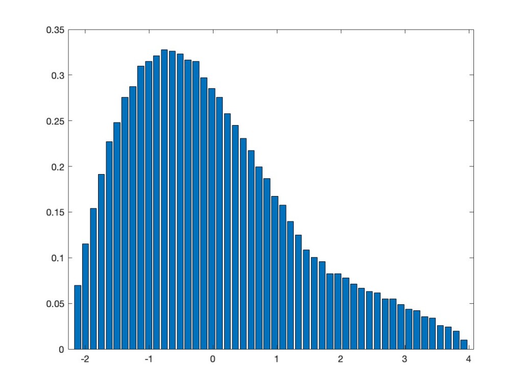
But now the Gaussian equivalence principle says that this $Y_N$ should asymptotically have the same distribution as the original matrix perturbed by a noise, i.e., as $\theta_1 X_N+\theta_2 Z_N$ , where $Z_N$ is a GOE matrix, independent from $X_N$ , and where in our case $\theta_1=1/2$ and $\theta_2=\sqrt{5(1-2/\pi)}/2$ . The following plot superimposes the eigenvalue distribution of $\theta_1 X_N+\theta_2 Z_N$ to the preceding plot for $Y_N$ . Looks convincing, doesn’t it.

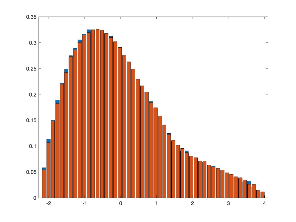
One should note that the ReLU functions does not fall into the class of (polynomial or analytic) functions, for which the results are usually proved, but ReLU is explicit enough, so that probably one could also do this more directly in this case. Anyhow, all this should just be an appetizer, there is still quite a bit to formulate and prove in this direction, but I am looking forward to a formidable feast in the end.

Berkeley’s Probabilistic Operator Algebra Seminar is Back

Leave a reply

Voiculescu’s online seminar on probabilistic operator algebra is running again, for the spring term, but now with a different time; it’s not on Mondays anymore, but on Tuesdays. For more info and details about the upcoming talks, see here. In particular, to get the zoom links for the talks, one should write to Jorge (jgarzav_at_caltech_dot_edu).

Actually, the next talk, on January 30 at 10:30 a.m. Pacific time (which is 7:30 p.m. German time), will be given by myself. It will be on Bi-free probability and reflection positivity and is based on my small note on the arXiv. Most of the talk will be about my (not very deep) understanding of the notion of reflection positivity, which has quite some relevance in quantum field theory and statistical physics. It seems to me that in the bi-free extension of free probability, we have a canonical candidate for a reflection, namely the exchange between the two (left and right) faces and it might be worth to investigate positivity questions in this context.

Free probability, between math and physics (and also machine learning) – some updates

1 Reply

In the recent post of a similar title I mentioned some papers which related physics problems (eigenstate thermalization hypothesis or Open Quantum SSEP) with free probability. Let me point out that the title of the preprint by Hruza and Bernard has been changed to “Coherent Fluctuations in Noisy Mesoscopic Systems, the Open Quantum SSEP and Free Probability” and that there are some new and follow up preprints in this directions, namely “Spectrum of subblocks of structured random matrices: A free probability approach“, by Bernard and Hruza, and also “Designs via free probability“, by Fava, Kurchan, Pappalardi. In all of them free cumulants and their relations to random matrices play an important role. Not too surprisingly, I find this very interesting in general, but also in particular, as during my voyage in the machine learning world I became a bit obsessed with the fact that free cumulants are given by the leading order of classical cumulants of the entries of unitarily invariant matrix ensembles (with a “cyclic” or “loop” structure of the indices). This seems to be highly relevant – though, at the moment I am not actually sure for what exactly.

Anyhow, if anybody is interested in this, in the last lecture of my machine learning course I give a very high level survey on these relations, and in the video on Gaussian equivalence principle in the same course I talk about a more concrete model of this in the random features model context.

Free Probability, Random Matrices and Machine Learning

1 Reply

Update (August 14): The lecture notes of the course on “High-Dimensional Analysis: Random Matrices and Machine Learning” are now available.

My activity on this blog has been quite low for a while, so it might be good to give a life sign and let you know that I still intend to keep the blog running, and hopefully be more active again in the future.

Lately, I have become interested in machine learning, mostly from the point of view of random matrices and free probability. I am trying to get some ideas what is going on there on a mathematical and conceptual level – mostly from the perspective that neural networks should give some inspirations for interesting questions on and extensions of random matrix and free probability theory.

The best way to learn a subject is to teach it, and that’s what I did. I just finished here in Saarbrücken a lecture series on “High-Dimensional Analysis: Random Matrices and Machine Learning”. I have created a blog page concerning this course; the lectures were recorded and will bit by bit be uploaded to the corresponding youtube playlist.

I hope to have more to say here on those topics in the (hopefully not too far) future. I know that quite a few people from our community have also some interest (maybe even already some work) in this direction. Guest blogs on such topics are highly welcome!

Free Probability Theory

A blog on freeing probability from its commutative chains

A Story of the Determinant of Operator-Valued Semicircular Elements

Doing Mathematics with AI — but How?

The intermediate quantum permutation group problem

Understanding Non-Linearity in Random Matrices

The noncommutative Edmonds’ problem revised: how to calculate the inner rank of matrices in noncommuting variables

What do determinants tell us about the eigenvalues of integer-valued matrices? — And what can we say about Fuglede-Kadison determinants of operator-valued semicircular elements?

“Structured random matrices and cyclic cumulants: A free probability approach” by Bernard and Hruza

Berkeley’s Probabilistic Operator Algebra Seminar is Back

Free probability, between math and physics (and also machine learning) – some updates

Free Probability, Random Matrices and Machine Learning