Update: I will give an online talk on my work with Alex in Voiculescu’s Probabilistic Operator Algebra Seminar on Monday, Feb 3, at 9am Pacific time (which is 6pm German time). In order to get the online link for the talk you should write to jgarzav at caltech dot edu.
What is this about? Consider a random matrix ensemble XN which has a limiting eigenvalue distribution for N going to infinity. In the machine learning context applying non-linear functions to the entries of such matrices plays a prominent role and the question arises: what is the asymptotic effect of this operation. There are a couple of results in this direction; see, in particular, the paper by Pennington and Worah and the one of Peche. However, it seems that they deal with quite special choices for XN, like a product of two independent Wishart matrices. In those cases the asymptotic effect of applying the non-linearity is the same as taking a linear combination of the XN with an independent Gaussian matrix. The coefficients in this linear combination depend only on a few quantities calculated from the non-linear function. Such statements are often known as Gaussian equivalence principle.
Our main contribution is that this kind of result is also true much more generally, namely for the class of rotationally invariant matrices. The rotational invariance is kind of the underlying reason for the specific form of the result. Roughly, the effect of the non-linearity is a small deformation of the rotational invariance, so that the resulting random matrix ensemble still exhibits the main features of rotational invariance. This provides precise enough information to control the limiting eigenvalue distribution.
We consider the real symmetric case, that is, symmetric orthogonally invariant random matrices. Similar results hold for selfadjoint unitarily invariant random matrices, or also for corresponding random matrices without selfadjointness conditions.
In addition to what I already showed in the above mentioned previous post, we extended the results now also to a multi-variate setting. This means we can also take, again entrywise, a non-linear function of several jointly orthogonally invariant random matrices. The asymptotic eigenvalue distribution after applying such a function is the same as for a linear combination of the involved random matrices and an additional independent GOE. As an example, take the two random matrices XN=AN2– BN and YN=AN4+CNAN+ANCN, where AN, BN, CN are independent GOEs. Note that, by the appearance of AN in both of them, they are not independent, but have a correlation. Nevertheless, they are jointly orthogonally invariant — that is, the joint distribution of all their entries does not change if we conjugate both of them by the same orthogonal matrix. We consider now the non-linear random matrix max(XN,YN), where we take entrywise the maximum of the corresponding entries in XN and YN. Our results say that asymptotically this should have the same eigenvalue distribution as the linear model aXN+ bYN + cZN, where ZN is an additional GOE, which is independent from AN, BN, CN, and where a, b, c are explicitly known numbers. The next plot superimposes the two eigenvalue distributions.
Let me first recall the noncommutative Edmonds’ problem. Consider a matrix
,
where the are noncommuting variables and the are arbitrary matrices of the same size N; N is fixed, but arbitrary.
The noncommutative Edmonds’ problem asks whether A is invertible over the noncommutative rational functions in the ; this is equivalent (by deep results of Cohn) to asking whether A is full, i.e., its noncommutative rank is equal to N. The noncommutative rank is here the inner rank rank(A), i.e., the smallest integer r such that we can write A as a product of an Nxr and an rxN-matrix. This fullness of the inner rank can also be equivalently decided by a more analytic object: to the matrix A we associate a completely positive map
In terms of , the fullness condition for A is equivalent to the fact that is rank non-decreasing (here we have of course the ordinary commutative rank on the complex NxN-matrices).
This noncommutative Edmonds’ problem has become quite prominent in recent years and there are now a couple of deterministic algorithms; see, in particular, the work of Garg, Gurvits, Oliveira and Widgerson.
Let me now recall our noncommutative probabilistic approach to the noncommutative Edmonds’ problem, by replacing the formal variables by concrete operators on infinite-dimensional Hilbert spaces. And a particular nice, and our favorite, choice for the analytic operators are freely independent semicircular variables , which are the noncommutative analogues of independent Gaussian random variables. In the case where all the are selfadjoint, the matrix
is a matrix-valued semicircular element.
Since one can reduce the general case to the selfadjoint one, it suffices to consider in the following the selfadjoint situation. Then the corresponding S is also a selfadjoint operator, hence its distribution is a probability measure on the real line. By our work of the last ten years or so we know that the invertibility of the formal matrix A over the noncommutative rational functions is equivalent to the invertibility of S as an unbounded operator. But this is equivalent to the question whether S has a trivial kernel, which is equivalent to the question whether its distribution has no atom at zero.
And we know how to calculate the distribution of our matrix-valued semicircular element S. Namely its Cauchy transform g(z), that is, the analytic function
on the complex upper half plane is of the form
where G(z) is given as the unique solution of the matrix-valued equation
,
in the lower half-plane of the NxN-matrices. One should note that for each z in the upper complex half plane there is (by some old results of mine with Reza Rashidi Far and Bill Helton) exactly one solution G(z) in the complex lower half-plane of the matrices. And, finally, we know that can have an atom only at zero, and the inner rank of A is related to the mass of this atom; more precisely,
So it seems, problem solved: Calculate the Cauchy transform and use the Stieltjes inversion formula to get the mass of the distribution at zero. We can even make this very concrete; what we need to consider is
in the limit where the positive real number y tends to zero. This limit is the mass of the atom at zero.
This is nice, but of course we cannot calculate anything analytically here, but have to rely on numerical approximations. So the question is, for which y should we calculate with which accuracy to be able to make a justified statement about the mass of the atom. And this is were things are getting tricky, but also nice.
Consider, for example, the matrix-valued semicircular element
If you want to know how we can get out of our machinery that the atom at zero of its distribution has mass 0.5 (that is, its noncommutative rank is 2), have a look at the revised version of our paper!
How can we convince ourselves that there are no two eigenvalues close to zero; say, you should convince me that two eigenvalues both with absolute value smaller than 0.1 are not possible. Of course, we should not calculate the eigenvalues but decide on this by arguments as soft as possible.
It is easy to get upper bounds for eigenvalues by the operator norm or the normalized trace of the matrix – those are quantities which are usually easy to control.
Not so clear are lower bounds, but actually it’s the determinant which will be of good use here. Namely, since the determinant is the product of the eigenvalues, knowing a lower bound for the absolute value of the determinant, together with the above mentioned easy upper bounds, gives lower bounds for the absolute values of the non-zero eigenvalues. In this example, we can calculate the determinant as -1, estimate the norm against the Frobenius norm of and can derive from this that no two eigenvalues of absolute value smaller than 0.1 are possible, because otherwise we would have the following estimate
which contradicts the fact that .
Maybe you don’t like so much the idea of having to calculate the determinant, as this does not feel so soft. Assume however that I told you, as an oracle, that the matrix is invertible, then you can forget about calculating the determinant and just argue that the determinant of a matrix with integer entries must be an integer, too, and since it cannot be zero you can conclude that it must in absolute value at least be 1; and so you can repeat the above estimate.
Those observations are of course not restricted to the above concrete example; actually, I have hopefully convinced you that no invertible matrix with integer entries can have too many eigenvalues close to zero, and the precise estimate depends on the matrix only through its operator norm.
This kind of reasoning can actually be extended to “infinite-dimensional matrices”, which means for us operators in a finite von Neumann algebra. There we are usually interested in the distribution of selfadjoint operators with respect to the trace and in recent work with Johannes Hoffmann and Tobias Mai it has become important to be able to decide that such distributions do not accumulate too much mass in a neighborhood of zero. In finite von Neumann algebras there exists also a nice version of the determinant, named after Fuglede and Kadison, and the main question is whether the above reasoning survives also in such a setting. And indeed, it does for the operators in which we are interested. But this is for reasons which are still nice, but quite a bit more tricky than for ordinary matrices.
The operators we are interested in are operator-valued semicircular elements of the form , where the are free semicircular elements and the are ordinary mxm matrices, with the only restriction that their entries are integers. We assume that such an S is invertible (as an unbounded operator) ; one can show that then its Fuglede-Kadison determinant is not equal to zero. The main question is whether we have a uniform lower estimate for away from zero. As there is now no formula for the determinant in terms of the entries of the matrix S, the integer values for the entries of the are of no apparent use. Still we are able to prove the astonishing fact that for all such invertible operator-valued semicircular operators their Fuglede-Kadison determinant is always .
For all this and much more you should have a look at my newest paper Fuglede-Kadison determinants of matrix-valued semicircular elements and capacity estimates with Tobias. If you need more of an appetizer, here is also the abstract of this paper: We calculate the Fuglede-Kadison determinant of arbitrary matrix-valued semicircular operators in terms of the capacity of the corresponding covariance mapping. We also improve a lower bound by Garg, Gurvits, Oliveira, and Widgerson on this capacity, by making it dimension-independent.
If this is still not enough to get you interested, maybe a concrete challenge will do. Here is a conjecture from our work on the limiting behavior of determinants of random matrices.
Conjecture: Let m and n be natural numbers and, for each i=1,…,n, an mxm-matrix with integer entries be given. Denote by the corresponding completely positive map
Assume that is rank non-decreasing. Then consider n independent GUE random matrices and let denote the Gaussian block random matrix
of size mN x mN. We claim that is invertible for sufficiently large N and that
where the capacity is defined as the infimum of over all for which det(b)=1.
The evolution of some papers of Bernard and Hruza in the context of “Quantum Symmetric Simple Exclusion Process” (QSSEP) have been addressed before in some posts, here and here. Now there is a new version of the latest preprint, with the more precise title “Structured random matrices and cyclic cumulants : A free probability approach“. I think the connection of the considered class of random matrices with our free probability tools (in particular, the operator-valued ones) is getting nicer and nicer. One of the new additions in this version is the proof that applying non-linear functions entrywise to the matrices (as is usually done in the machine learning context) does not lead out of this class and one can actually describe the effect of such an application.
I consider all this as a very interesting new development which connects to many things, and I will try to describe this a bit more concretely in the following.
For the usual unitarily invariant matrix ensembles we know that the main information about the entries which contributes in the limit to the calculation of the matrix distribution are the cyclic classical cumulants (or ”loop expectation values”). Those are cumulants of the entries with cyclic index structure – and, for the unitarily invariant ensembles, the asymptotics of those cumulants does not depend on the chosen indices . Actually, in the limit, with the right scaling, those give the free cumulants of our limiting matrix distribution. The idea of Bernard and Hruza is now to extend this to an inhomogeneous setting, where the indices matter and thus the limiting information is given by ”local” free cumulants where the are the limits of . For the operator-valued aficionado this has the flavor of operator-valued cumulants (over the diagonals), and this is indeed the case, as shown in the paper. For the case of inhomogeneous Gaussian matrices, where the limits are given by operator-valued semicircular elements, such results are not new, going back to the work of Dima Shlyakhtenko on band matrices, and constitute one of our most beloved indications for the power of operator-valued free probability. The paper of Bernard and Hruza goes much beyond the semicircular case and opens a very interesting direction. The fact that this is motivated by problems in statistical physics makes this even more exciting. Of course, there are many questions arising from this, on which we should follow up. In particular, is there a good version of this not only over diagonal matrices; or, is there a relation with the notion of R-cyclic distributions, which I introduced with Andu and Dima a while ago in this paper?
As I mentioned at the beginning I am also intrigued by the effect of applying non-linear functions to the entries of our matrices. This is something, we usually don’t do in ”classical” random matrix theory, but which has become quite popular in recent years in the machine learning context. There are statements which go under the name of Gaussian equivalence principle, which say that the effect of the non-linearity is in many cases the same as adding an independent Gaussian random noise. Actually, this is usually done for special random matrices, like products of Wishart matrices. However, this seems to be true more general; I was convinced that this is valid for unitarily invariant matrices, but the paper of Bernard and Hruza shows that even in their more general setting one has results of this type.
In order to give a concrete feeling of what I am talking about here, let me give a concrete numerical example for the unitarily invariant case. Actually, I prefer her the real setting, i.e., orthogonal invariant matrices. For me canonical examples of those are given by polynomials in independent GOE, so let us consider here , where and are independent GOE. The following plot shows the histogram of the eigenvalues of one realization of for $N=5000$.
We apply now a non-linear function to the entries of . Actually, one has to be a bit careful about what this means; in particular, one needs a good scaling and should not act naively on the diagonals, as this would otherwise dominate everything. Here is the precise definition of the entries of the new matrix .
For the function f, let’s take the machine learning favorite, namely the ReLU function, i.e., . Here is the histogram of the eigenvalues of the corresponding matrix
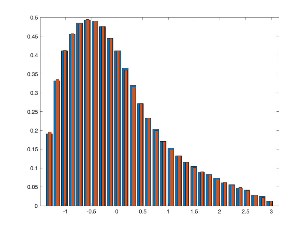
But now the Gaussian equivalence principle says that this should asymptotically have the same distribution as the original matrix perturbed by a noise, i.e., as , where is a GOE matrix, independent from , and where in our case and . The following plot superimposes the eigenvalue distribution of to the preceding plot for . Looks convincing, doesn’t it.
One should note that the ReLU functions does not fall into the class of (polynomial or analytic) functions, for which the results are usually proved, but ReLU is explicit enough, so that probably one could also do this more directly in this case. Anyhow, all this should just be an appetizer, there is still quite a bit to formulate and prove in this direction, but I am looking forward to a formidable feast in the end.
Voiculescu’s online seminar on probabilistic operator algebra is running again, for the spring term, but now with a different time; it’s not on Mondays anymore, but on Tuesdays. For more info and details about the upcoming talks, see here. In particular, to get the zoom links for the talks, one should write to Jorge (jgarzav_at_caltech_dot_edu).
Actually, the next talk, on January 30 at 10:30 a.m. Pacific time (which is 7:30 p.m. German time), will be given by myself. It will be on Bi-free probability and reflection positivity and is based on my small note on the arXiv. Most of the talk will be about my (not very deep) understanding of the notion of reflection positivity, which has quite some relevance in quantum field theory and statistical physics. It seems to me that in the bi-free extension of free probability, we have a canonical candidate for a reflection, namely the exchange between the two (left and right) faces and it might be worth to investigate positivity questions in this context.
In the recent post of a similar title I mentioned some papers which related physics problems (eigenstate thermalization hypothesis or Open Quantum SSEP) with free probability. Let me point out that the title of the preprint by Hruza and Bernard has been changed to “Coherent Fluctuations in Noisy Mesoscopic Systems, the Open Quantum SSEP and Free Probability” and that there are some new and follow up preprints in this directions, namely “Spectrum of subblocks of structured random matrices: A free probability approach“, by Bernard and Hruza, and also “Designs via free probability“, by Fava, Kurchan, Pappalardi. In all of them free cumulants and their relations to random matrices play an important role. Not too surprisingly, I find this very interesting in general, but also in particular, as during my voyage in the machine learning world I became a bit obsessed with the fact that free cumulants are given by the leading order of classical cumulants of the entries of unitarily invariant matrix ensembles (with a “cyclic” or “loop” structure of the indices). This seems to be highly relevant – though, at the moment I am not actually sure for what exactly.
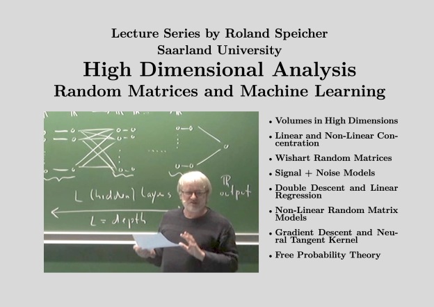
Update (August 14): The lecture notes of the course on “High-Dimensional Analysis: Random Matrices and Machine Learning” are now available.
My activity on this blog has been quite low for a while, so it might be good to give a life sign and let you know that I still intend to keep the blog running, and hopefully be more active again in the future.
Lately, I have become interested in machine learning, mostly from the point of view of random matrices and free probability. I am trying to get some ideas what is going on there on a mathematical and conceptual level – mostly from the perspective that neural networks should give some inspirations for interesting questions on and extensions of random matrix and free probability theory.
The best way to learn a subject is to teach it, and that’s what I did. I just finished here in Saarbrücken a lecture series on “High-Dimensional Analysis: Random Matrices and Machine Learning”. I have created a blog page concerning this course; the lectures were recorded and will bit by bit be uploaded to the corresponding youtube playlist.
I hope to have more to say here on those topics in the (hopefully not too far) future. I know that quite a few people from our community have also some interest (maybe even already some work) in this direction. Guest blogs on such topics are highly welcome!
Hawking famously showed that black holes radiate just like a blackbody. Behaving like a thermodynamic object, a black hole has an entropy worth a quarter of its area (in units of the Planck area), which is now known as the Bekenstein-Hawking (BH) entropy. Through several thought experiments, Bekenstein already reached this conclusion up to the 1/4 prefactor before Hawking’s calculation, and he also reasoned that a black hole is the most entropic object in the universe in the sense that one cannot pack entropy more efficiently in a region bounded by the same area with the same mass than a black hole does. This is known as the Bekenstein bound. As for Hawking, the BH entropy can be deduced from the gravity partition function computed using the gravitational path integral (GPI), just like how entropy is derived from the partition function in statistical physics.
However, Hawking’s discovery led to a new problem that put the fundamental principle of physics in question, that the information carried by a closed system cannot be destroyed under evolution. This cherished principle is respected by the unitarity in quantum theory. On the other hand, since the radiation has a relatively featureless thermal spectrum, it cannot preserve all the information a star contains before it collapses into a black hole nor the information carried by the objects that later fall into it. If the radiation is all there is after the complete evaporation, the information is apparently lost. If we are not willing to give up our well-established theories, one way out is to speculate that the black hole never really evaporates away but it somehow stops evaporating and becomes a long-living remnant when it has shrunk to the Planckian size. All the entropy production is then due to the correlation with the remaining black hole. While this could be plausible, there is already tension long before the black hole approaches its end life. If we examine the radiation entropy after the black hole passes its half-life, the radiation entropy keeps rising according to Hawking and they have to be attributed to the correlation with the remaining black hole. This means that the mid-aged black hole has to be as entropic as the radiation but this is impossible without violating the Bekenstein bound. In fact, Page famously argued that if we suppose a black hole indeed operates with some unknown unitary evolution, then typically the radiation entropy should start to go down at its half-life, in contrast to Hawking’s calculation. We refer to this tension past the Page time as the entropic information puzzle. The challenge is to derive the entropy curve that Page predicted, i.e. the Page curve, using a first-principle gravity calculation.
Recently, significant progress (see here and here ) has been made to resolve the entropic information puzzle. (cf. this review article and the references therein.) The entropy of radiation is calculated in semiclassical gravity with GPI à la Hawking, and the Page curve is derived. Remarkably and unexpectedly, the Page curve can be obtained in the semiclassical regime without postulating radical new physics. The new ingredient is the replica trick, which essentially probes the radiation spectrum with many copies of the black hole. The idea is that we’d like to compute all the moments of the radiation density matrix , where we rewrite it as the expectation value of the n-fold swap operator on n identical and independent replicas of the state . The trouble is we don’t know explicitly what is, rather our current understanding of quantum gravity only allows us to describe the moments we’d like to compute implicitly in terms of a n-replica partition function with appropriately chosen boundary conditions.
where the LHS is what we really compute in gravity and we postulate on the RHS that this partition function gives the moments of that we want.
To evaluate , the GPI sums over all legit configurations, such as all sorts of metrics, topologies, and matter fields, consistent with the given boundary conditions. In particular, new geometric configurations show up and modify Hawking’s result. These geometries connect different replicas and are called replica wormholes. Since Hawking only ever considered a single black hole scenario, he missed these wormhole contributions in his calculation. In practice, performing the GPI over all the wormhole configurations can be technically difficult and one needs to resort to some simplifications and approximations. For the entropy calculation, one often drops all the wormholes but the maximally symmetric one that connects all the replicas. This approximation leads to a handy formula, called the island formula, for computing the radiation entropy and thus the Page curve. However, we should keep in mind that sometimes this approximation can be bad and the island formula needs a large correction. It would be interesting to see when and how this happens.
Fortunately, there is a toy model of an evaporating black hole due to Penington-Shenker-Stanford-Yang (PSSY), in which one can resolve the spectrum of the radiation density matrix without compromise. This model simplifies the technical setup as much as possible while still keeping the essence of the entropic information puzzle. This recent paper computes the radiation entropy by implementing the full GPI and identifies the large corrections to the commonly used island formula. Interestingly, the key ingredient is free probability. The GPI becomes tractable after being translated into the free probabilistic language. Here we summarise the main ideas. In the replica trick GPI, the wormholes are organized by the non-crossing partitions. Feynman taught us to sum over all contributions weighted by the exponential of the gravity action evaluated on the wormholes (wormhole contributions). Then the resulting n-replica partition function (i.e. nth moment of ), is equal to summing over the wormhole contributions, matching exactly with the free moment-cumulant relation. Therefore, the wormhole contributions shall be treated as free cumulants. Furthermore, the matter field propagating on a particular wormhole configuration (labeled by ) is organized by the Kreweras complement of . Together the total contribution to the n-replica partition function from both the wormholes and the matter field on them amounts to a free multiplicative convolution. It is a convolution between two implicit probability distributions encoding the quantum information from the gravity sector and the matter sector. With this observation, one can then evaluate the free multiplicative convolution using tools from free harmonic analysis to resolve the radiation spectrum and thus the Page curve.
The figure illustrates a typical configuration for 13 replica black holes. The arrowed solid lines with length indicate the boundary conditions that prepare each black hole in a thermal state of temperature ; the dashed lines indicate the radiation quanta and they are cyclically connected to implement the observable . Combinatorially, any wormhole configuration (in black) corresponds to a non-crossing partition and the configuration of the matter fields (in red) corresponds to the corresponding Kreweras complement.
Through modeling the free random variables in random matrices, we can go one step further and deduce from the convolution that the radiation spectrum matches the one obtained from a generalized version of Page’s model. Therefore, we really start from the first-principle gravity calculation to address the challenge that Page posed, and free probability helps to make this connection clear and precise in the context of the PSSY model. What remains to be understood is why freeness is relevant here in the first place. To what extent is free probability useful in quantum gravity and is there a natural reason for freeness to emerge? Free probability already has applications in quantum many-body physics (cf. the previous post). If we think of quantum gravity as a quantum many-body problem, some aspects of it can be understood in terms of random tensor networks. This viewpoint has been very successful in the context of the AdS/CFT correspondence. In this view, freeness can plausibly be ubiquitous in gravity thanks to the random tensors. Another hint comes from concrete quantum mechanic models such as the SYK model, from which simple gravity theory can emerge in the low energy regime. The earlier work of Pluma and Speicher drew the connection between the double-scaled SYK model and the q-Brownian motion. Perhaps quantum gravity is calling for new species of non-commutative probability theories that differ from the usual quantum theory.
There is a subtle logical inconsistency that we should address. The postulate above is not exactly correct. The free convolution indicates that the radiation spectrum obtained is generically continuous, suggesting that we are dealing with a random radiation density matrix. Hence, in hindsight, it’s more appropriate to say that the GPI is computing the expected n-th moment . However, it is puzzling because this extra ensemble average radically violates the usual Born’s rule in quantum physics.
In fact, we can give a proper physical explanation within the standard quantum theory. This was pointed out in this other recent paper, leveraging the power of the quantum de Finetti theorem. The key is to make a weaker postulate that the implicit state upon which we evaluate should be correlated instead of independent among the n replicas. Let’s denote this joint radiation state as , which may not be a product state as postulated above. This is because in the GPI , one only imposes the boundary conditions, so gravity could automatically correlate the state in the bulk even if one means to prepare them independently. It’s hence too strong to postulate that the joint radiation state implicitly defined via the boundary conditions has the product form . Nonetheless, this joint state should still be permutation-invariant because we don’t distinguish the replicas. Even better, it should also be exchangeable (meaning that the quantum state can be treated as a marginal of a larger permutation-invariant state) because we can in principle consider an infinite amount of replicas and randomly sample n replicas to evaluate . This allows us to invoke the de Finetti theorem to deduce that the joint radiation state on n-replicas is a convex combination over identical and independent replica states with some probability measure .
.
The de Finetti theorem thus naturally brings in an ensemble average that is consistent with the result of the free convolution calculation. Interestingly, one can further show that the de Finetti theorem implies that the replica trick really computes the regularized entropy , i.e. the averaged radiation entropy of infinitely many replica black holes. It is to be contrasted with the radiation entropy of a single black hole, which can be much bigger because of the uncertainty in the measure . The latter is closer to what Hawking calculated and he was wrong because the entropy contribution due to probability measure is not what we are after. This ensemble reflects that our theory of quantum gravity is incomplete to correctly pin down the exact description of the radiation, but we really shouldn’t attribute this uncertainty to the physical entropy of radiation. The gist of the replica trick is that with many copies the contribution from is moderated out in the regularized entropy because it doesn’t scale with the number of replicas. Therefore, when someone actually goes out and operationally measures the radiation entropy, she has to prepare many copies of the black hole and sample them to deduce the measurement statistics just like for measuring any quantum observable. Then she will find herself dealing with a de Finetti state, where acts like a Bayesian prior that reflects our ignorance of the fundamental theory. Nonetheless, the measurement shall reveal the truth and help update the prior to peak at some particular . Hence, operationally the entropy measured should never depend on how uncertain the prior is. This is perhaps a better explanation of what Hawking did wrong. These conceptual issues are now clarified thanks to the wisdom of de Finetti.
The fun of free probability is that if you think you have seen everything in the subject suddenly new exciting connections are popping up. This happened for example a few months ago with the preprints
According to the authors, the occurrence of free probability in both problems has a similar origin: the coarse-graining at microscopic either spatial or energy scales, and the unitary invariance at these microscopic scales. Thus the use of free probability tools promises to be ubiquitous in chaotic or noisy many-body quantum systems.
I still have to have a closer look on these connections and thus I am very excited that there will be great opportunity for learning more about this (and other connections) and discussing it with the authors at a special day at IHP, Paris on 25 January 2023. This is part of a two-day conference “Inhomogeneous Random Structures”.
Wednesday 25 January: Free probability, between maths and physics. Moderator: Jorge Kurchan (Paris)
Free probability is a flourishing field in probability theory. It deals with non-commutative random variables where one introduces the concept of «freeness» in analogy to «independence» of commuting random variables. On the mathematical side, it has given new tools and a deeper insight into, amongst others, the field of random matrices. On the physics side, it has recently appeared naturally in the context of quantum chaos, where all its implications have not yet been fully worked out.
Speakers: Denis Bernard (Paris), Jean-Philippe Bouchaud (Paris), Laura Foini (Saclay), Alice Guionnet (Lyon), Frederic Patras (Nice), Marc Potters (Paris), Roland Speicher (Saarbrücken)
There is presently quite some activity around the q-Gaussians, about which I talked in my last post. Tomorrow (i.e., on Monday, April 25) there will be another talk in the UC Berkeley Probabilistic Operator Algebra Seminar on this topic. Mario Klisse from TU Delft will speak on his joint paper On the isomorphism class of q-Gaussian C∗-algebras for infinite variables with Matthijs Borst, Martijn Caspers and Mateusz Wasilewski. Whereas my paper with Akihiro deals only with the finite-dimensional case (and I see not how to extend this to infinite d) they deal with the infinite-dimensional case, and, quite surprisingly, they have a non-isomorphism result: namely that the C*-algebras for q=0 and for other q are not isomorphic. This makes the question for the von Neumann algebras even more interesting. It still could be that the von Neumann algebras are isomorphic, but then by a reason which does not work for the C*-algebras – this would be in contrast to the isomorphism results of Alice and Dima, which show the isomorphism of the von Neumann algebras (for finite d and for small q) by actually showing that the C*-algebras are isomorphic.
I am looking forward to the talk and hope that afterwards I have a better idea what is going on – so stay tuned for further updates.


 ,
, are noncommuting variables and the
  are arbitrary matrices of the same size N; N is fixed, but arbitrary.
 , the fullness condition for A is equivalent to the fact that
  , which are the noncommutative analogues of independent Gaussian random variables. In the case where all the
 of our matrix-valued semicircular element S. Namely its Cauchy transform g(z), that is, the analytic function

 ,
,

 with which accuracy to be able to make a justified statement about the mass of the atom. And this is were things are getting tricky, but also nice.

 and can derive from this that no two eigenvalues of absolute value smaller than 0.1 are possible, because otherwise we would have the following estimate
 .
. , where the
  are free semicircular elements and the
  is not equal to zero. The main question is whether we have a uniform lower estimate for
  .
.
 and let
  denote the Gaussian block random matrix

 is defined as the infimum of
  over all
  for which det(b)=1.
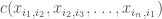 – and, for the unitarily invariant ensembles, the asymptotics of those cumulants does not depend on the chosen indices
  . Actually, in the limit, with the right scaling, those give the free cumulants
  of our limiting matrix distribution. The idea of Bernard and Hruza is now to extend this to an inhomogeneous setting, where the indices matter and thus the limiting information is given by ”local” free cumulants
  where the
  are the limits of
  . For the operator-valued aficionado this has the flavor of operator-valued cumulants (over the diagonals), and this is indeed the case, as shown in the paper. For the case of inhomogeneous Gaussian matrices, where the limits are given by operator-valued semicircular elements, such results are not new, going back to the
  , where
  are independent GOE. The following plot shows the histogram of the eigenvalues of one realization of
  for $N=5000$.
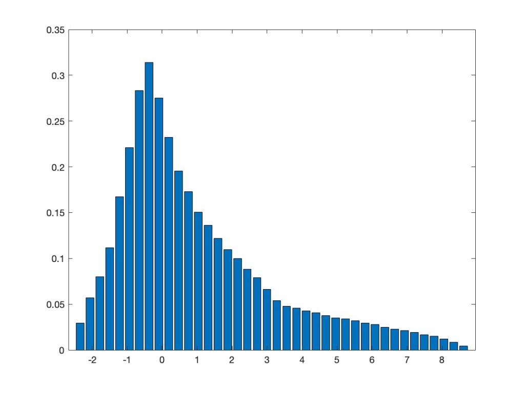
 .
.
 . Here is the histogram of the eigenvalues of the corresponding matrix
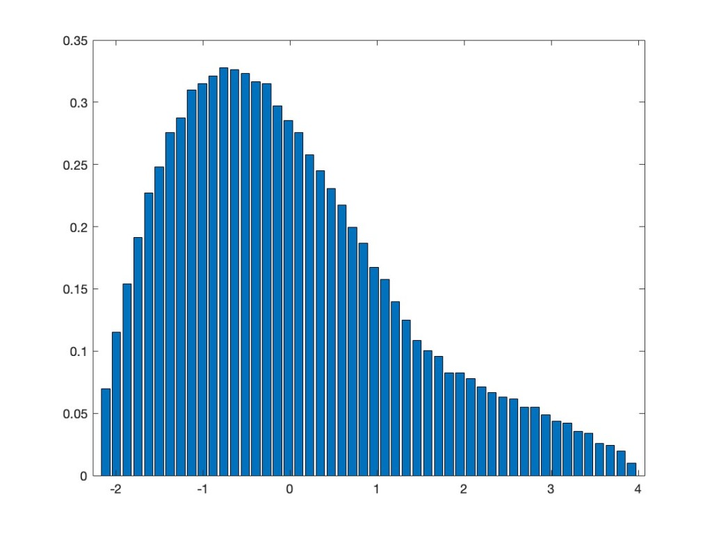
 , where
  is a GOE matrix, independent from
  and
and  . The following plot superimposes the eigenvalue distribution of
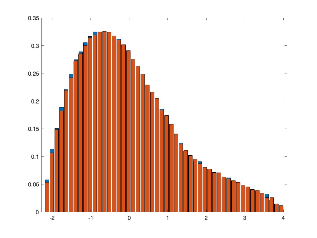
 , where we rewrite it as the expectation value of the n-fold swap operator
  on n identical and independent replicas of the state
  . The trouble is we don’t know explicitly what
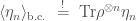
 , the GPI sums over all legit configurations, such as all sorts of metrics, topologies, and matter fields, consistent with the given boundary conditions. In particular, new geometric configurations show up and modify Hawking’s result. These geometries connect different replicas and are called replica wormholes. Since Hawking only ever considered a single black hole scenario, he missed these wormhole contributions in his calculation. In practice, performing the GPI over all the wormhole configurations can be technically difficult and one needs to resort to some simplifications and approximations. For the entropy calculation, one often drops all the wormholes but the maximally symmetric one that connects all the replicas. This approximation leads to a handy formula, called the island formula, for computing the radiation entropy and thus the Page curve. However, we should keep in mind that sometimes this approximation can be bad and the island formula needs a large correction. It would be interesting to see when and how this happens.
 ) is organized by the Kreweras complement of
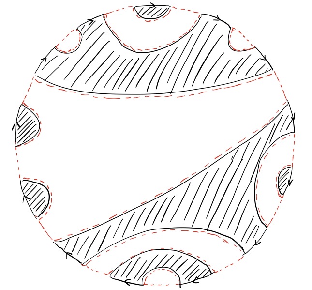
 indicate the boundary conditions that prepare each black hole in a thermal state of temperature
  ; the dashed lines indicate the radiation quanta and they are cyclically connected to implement the observable
  . Combinatorially, any wormhole configuration (in black) corresponds to a non-crossing partition and the configuration of the matter fields (in red) corresponds to the corresponding Kreweras complement.
 . However, it is puzzling because this extra ensemble average
  radically violates the usual Born’s rule in quantum physics.
  , which may not be a product state
  as postulated above. This is because in the GPI
  with some probability measure
  .
. .
. that is consistent with the result of the free convolution calculation. Interestingly, one can further show that the de Finetti theorem implies that the replica trick really computes the regularized entropy
  , i.e. the averaged radiation entropy of infinitely many replica black holes. It is to be contrasted with the radiation entropy of a single black hole, which can be much bigger because of the uncertainty in the measure