
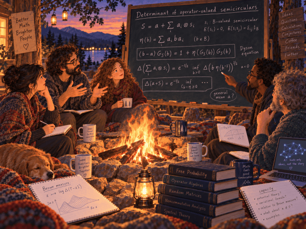
Operator-valued semicircular elements are the powerhouse of free probability and random matrix theory. In particular, the intrinsic freeness principle typically replaces random matrices by operator-valued semicircular elements and shows that, in many respects, the former are close to the latter. Thus it is important to understand as much as possible about operator-valued semicirculars.
An operator-valued semicircular element – say over – is of the form
where are free semicirculars. We denote by the normalized matrix trace on , and by the trace on the algebra, where the live. All information about such an element is contained in its mean
and its covariance
The covariance is a completely positive map from to .
We also know how, in principle, to calculate the distribution of . Its scalar-valued Cauchy transform is
This can be extracted from the operator-valued Cauchy transform
simply by
And is determined by the nice quadratic matrix-valued equation, usually called the Dyson equation,
So everything is determined by mean and covariance. Of course, some quantities are easier, others harder to extract in a meaningful way. For moments of , for example, one has the operator-valued free version of the Wick/Isserlis formula. The operator norm of , on the other hand, is not so easily accessible. In principle, this is given by the asymptotics of high moments, but that is not very concrete. So the following celebrated formula of Franz Lehner
comes as a nice surprise, as it reduces the upper spectral edge of the infinite-dimensional to a variational problem for the same quantity on the finite-dimensional matrix algebra . Here denotes the upper edge of the spectrum; for positive , Lehner’s original formulation gives the corresponding operator norm.
A few years ago together with Tobias Mai I was trying to understand the determinant (more precisely, the Fuglede–Kadison determinant) of an operator-valued semicircular element, in order to get some info about the accumulation of mass of the distribution of such a semicircular element close to zero. And we succeeded in finding a nice formula in terms of the covariance; more precisely the determinant was essentially given by the capacity of the covariance map. Capacity here is the quantity introduced by Gurvits in connection with operator scaling; it should not be confused with the various notions of channel capacity in quantum information. Unwinding this notion of capacity one can write our result concretely as
is here the Fuglede–Kadison determinant, which reduces in the finite-dimensional situation to
As you see, our result is only for mean . But in this case it has a striking similarity with Lehner’s formula:
And of course it raises the question: Can we extend our formula also to the case of general mean. We thought a little bit about this way back then, but did not see how to do this.
Now, in the times of AI hype, it is tempting to come back to this question and ask ChatGPT what it has to say on this. And actually, it has something to say. It proposes the following generalization
where
is the Hilbert-Schmidt inner product.
The condition means positivity as an operator on the Hilbert–Schmidt space , i.e.
ChatGPT also produces what it claims is a proof of all this — note that even the reduction of this to my formula with Tobias in the case of is non-trivial — and makes some remarks on the relevance for the Brown measure of an operator-valued circular element. Recall that the Brown measure of an operator is encoded by the logarithmic potential
So understanding determinants of shifted operators is exactly what one needs here.
All this looks somehow reasonable, but not very enlightening; and even if I had a Lean certificate for all this (which I don’t), I would still not be too satisfied.
So let’s talk about all this and hope that, together, we can get a better understanding of what is really going on.


Pingback: Doing Mathematics with AI — but How? | Free Probability Theory
That’s an interesting and refreshing approach for treating AI output. Okay, the Oracle has spoke and given us a piece of wisdom; now rather then autoformalize and get a certificate or iterate until we have a readable proof, let us gather together and digest it together, think about the meaning and interpret it for ourselves. Let us be humble, let us be students again. As an outsider to your field, I look forward to hearing how this goes.
On my own front: the Oracle filled the small missing piece in a puzzle I was trying to solve, it was a gem and easy to understand. I will probably write about this soon.
LikeLike
Pingback: The Story of the Determinant: Why the Determinant Formula is True | Free Probability Theory