Update: I will give an online talk on my work with Alex in Voiculescu’s Probabilistic Operator Algebra Seminar on Monday, Feb 3, at 9am Pacific time (which is 6pm German time). In order to get the online link for the talk you should write to jgarzav at caltech dot edu.
In the post “Structured random matrices and cyclic cumulants: A free probability approach” by Bernard and Hruza I mentioned the problem about the effect of non-linear functions on random matrices and showed some plots from my ongoing joint work with Alexander Wendel. Finally, a few days ago, we uploaded the preprint to the arXiv.
What is this about? Consider a random matrix ensemble XN which has a limiting eigenvalue distribution for N going to infinity. In the machine learning context applying non-linear functions to the entries of such matrices plays a prominent role and the question arises: what is the asymptotic effect of this operation. There are a couple of results in this direction; see, in particular, the paper by Pennington and Worah and the one of Peche. However, it seems that they deal with quite special choices for XN, like a product of two independent Wishart matrices. In those cases the asymptotic effect of applying the non-linearity is the same as taking a linear combination of the XN with an independent Gaussian matrix. The coefficients in this linear combination depend only on a few quantities calculated from the non-linear function. Such statements are often known as Gaussian equivalence principle.
Our main contribution is that this kind of result is also true much more generally, namely for the class of rotationally invariant matrices. The rotational invariance is kind of the underlying reason for the specific form of the result. Roughly, the effect of the non-linearity is a small deformation of the rotational invariance, so that the resulting random matrix ensemble still exhibits the main features of rotational invariance. This provides precise enough information to control the limiting eigenvalue distribution.
We consider the real symmetric case, that is, symmetric orthogonally invariant random matrices. Similar results hold for selfadjoint unitarily invariant random matrices, or also for corresponding random matrices without selfadjointness conditions.
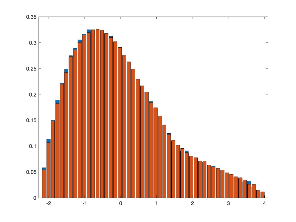
In addition to what I already showed in the above mentioned previous post, we extended the results now also to a multi-variate setting. This means we can also take, again entrywise, a non-linear function of several jointly orthogonally invariant random matrices. The asymptotic eigenvalue distribution after applying such a function is the same as for a linear combination of the involved random matrices and an additional independent GOE. As an example, take the two random matrices XN=AN2– BN and YN=AN4+CNAN+ANCN, where AN, BN, CN are independent GOEs. Note that, by the appearance of AN in both of them, they are not independent, but have a correlation. Nevertheless, they are jointly orthogonally invariant — that is, the joint distribution of all their entries does not change if we conjugate both of them by the same orthogonal matrix. We consider now the non-linear random matrix max(XN,YN), where we take entrywise the maximum of the corresponding entries in XN and YN. Our results say that asymptotically this should have the same eigenvalue distribution as the linear model aXN+ bYN + cZN, where ZN is an additional GOE, which is independent from AN, BN, CN, and where a, b, c are explicitly known numbers. The next plot superimposes the two eigenvalue distributions.
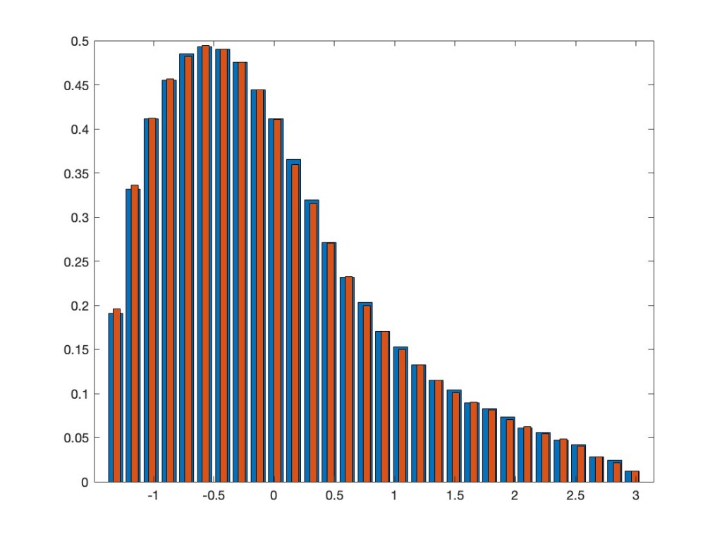
If you want to know more, in particular, why this is true and how the coefficients in the linear model are determined in terms of the non-linear function, see our preprint Entrywise application of non-linear functions on orthogonally invariant random matrices.
 – and, for the unitarily invariant ensembles, the asymptotics of those cumulants does not depend on the chosen indices
  . Actually, in the limit, with the right scaling, those give the free cumulants
  of our limiting matrix distribution. The idea of Bernard and Hruza is now to extend this to an inhomogeneous setting, where the indices matter and thus the limiting information is given by ”local” free cumulants
  where the
  are the limits of
  . For the operator-valued aficionado this has the flavor of operator-valued cumulants (over the diagonals), and this is indeed the case, as shown in the paper. For the case of inhomogeneous Gaussian matrices, where the limits are given by operator-valued semicircular elements, such results are not new, going back to the
  , where
  and
and  are independent GOE. The following plot shows the histogram of the eigenvalues of one realization of
  for $N=5000$.
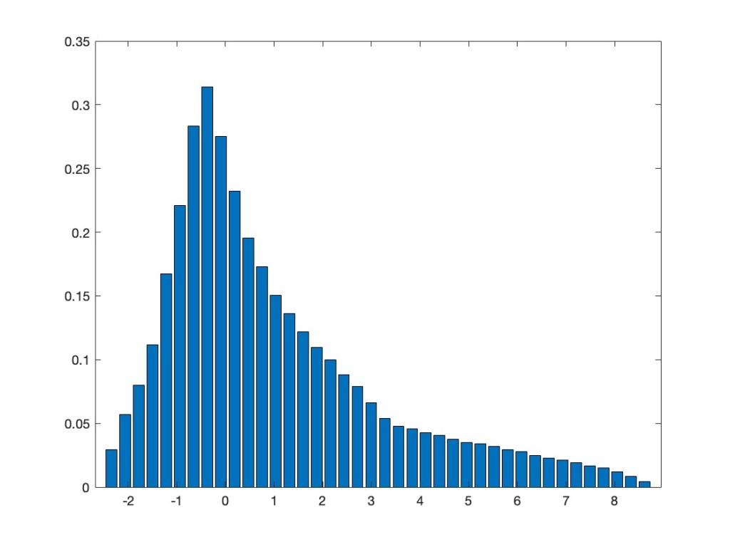
 .
.
 . Here is the histogram of the eigenvalues of the corresponding matrix
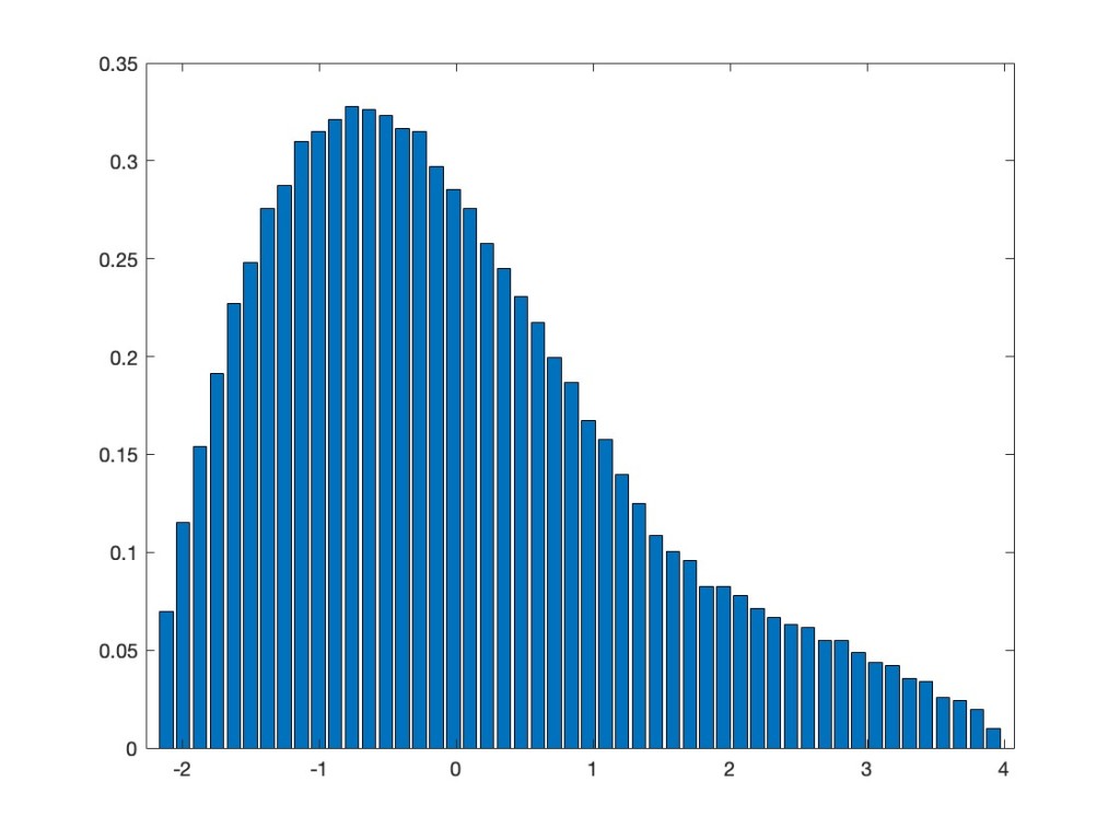
 , where
  is a GOE matrix, independent from
  and
and  . The following plot superimposes the eigenvalue distribution of